Category: Control Systems

We designed a speed controller for a real motor, the ABB Baldor-Reliance CDP3306 (¼ HP, 180 V, 1750 rpm), using only Python and its datasheet. The result settles a 1000 rpm step in 75 ms with no overshoot, a 76° phase margin, and a peak demand of 117 V from a 180 V drive.

Everything here uses open-source tools: python-control, NumPy, Matplotlib and pytest. The full script is built up section by section, and every number in the post comes from running it. This is the long-form companion to our Instagram carousel on the same build.

From datasheet to model parameters

Every model parameter traces back to a line in ABB’s customer information packet for the CDP3306. These are typical values, not guaranteed ones.

Datasheet field	Datasheet value	Model parameter
Armature voltage	180 V	Drive limit: 180 V
Base speed	1750 rpm	183 rad/s
Rated armature current	1.25 A	—
Armature resistance	8.54 Ω at 25 °C	R = 8.54 Ω
Armature inductance	60.59 mH	L = 60.6 mH
Voltage constant	98.01 V/krpm	K = 0.936 V·s/rad (= N·m/A)
Armature inertia	4.68 lb·in²	J = 1.37×10⁻³ kg·m²
No-load point	0.10 A at 1830 rpm	b = 4.88×10⁻⁴ N·m·s/rad

Two values need a short derivation:

• K is both the back-EMF constant and the torque constant in SI units: 98.01 V/krpm ÷ 104.7 = 0.936.
• b isn’t on the datasheet, but the no-load point gives it: b = K · I₀ / ω₀.

One datasheet catch: the online catalog listing gives the inertia as 4.68 lb·ft². The performance data sheet labels the same number LI² (lb·in²). The lb·ft² reading would mean 0.197 kg·m², which is physically impossible for an 11 kg motor, so we use lb·in². Always sanity-check your data before you design.

The motor model

Armature voltage in, shaft speed out: the DC motor is a second-order transfer function.

In python-control, with the datasheet constants:

import control as ct
import matplotlib.pyplot as plt
import numpy as np

# 1. Define physical motor constants (ABB Baldor-Reliance CDP3306 datasheet)
J = 1.37e-3   # Rotor moment of inertia (kg.m^2), 4.68 lb.in^2
b = 4.88e-4   # Motor viscous friction constant (N.m.s), from the no-load point
K = 0.936     # Motor torque & back-emf constant (N.m/A or V/rad/s), 98.01 V/krpm
R = 8.54      # Armature resistance (Ohm), at 25 C
L = 60.6e-3   # Armature inductance (H)

# Open-Loop Motor Transfer Function: armature voltage (V) -> speed (rad/s)
num_motor = [K]
den_motor = [J * L, (J * R) + (b * L), (b * R) + (K**2)]
motor_sys = ct.TransferFunction(num_motor, den_motor)

Before designing anything, check the model against the data:

• No-load speed: at 180 V the model predicts 1828 rpm. The datasheet measured 1830 rpm.
• Under load: across all seven load points on the datasheet, from 0.10 A to 1.68 A, the model’s speed stays within 1.3%. It droops slightly less than the real motor, because R rises as the winding warms.
• Poles: a lightly damped pair at −70.6 ± 74.9j rad/s. The electrical and mechanical time constants (7.1 ms and 13.4 ms) are close enough to interact.

Validate against data before you tune a single gain.

Requirements first

Write the requirements down before tuning anything, each one measurable so it can become a test later.

ID	Requirement	Target
REQ-01	Overshoot	≤ 5%
REQ-02	Settling time (2% band)	≤ 100 ms
REQ-03	Steady-state error	0
REQ-04	Phase margin	≥ 60°
REQ-05	Peak armature voltage for a 1000 rpm step	≤ 180 V

REQ-05 is the one most designs forget: the drive can’t supply more than 180 V, whatever the controller asks for.

The controller: PI on the error, D on the speed

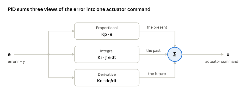
The P and I terms act on the error, as usual. The D term acts only on the measured speed, so a step in the setpoint never passes through the derivative.

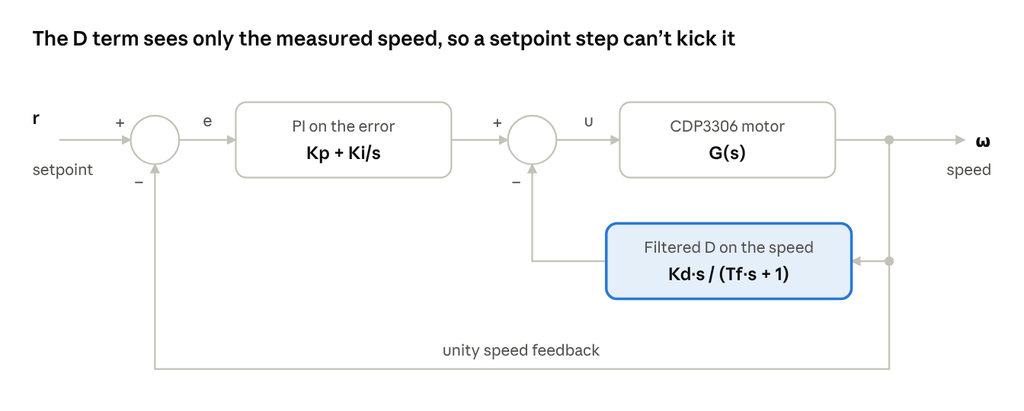
In code, PI sits in the forward path and the filtered D sits in an inner feedback loop around the motor:

# 2. Define PID Gains
Kp = 1.0     # Proportional Gain
Ki = 60.0    # Integral Gain
Kd = 0.002   # Derivative Gain
Tf = 0.002   # Derivative filter time constant (s)

# 3. Forward path controller (PI action on the error)
# C_pi(s) = Kp + Ki/s = (Kp*s + Ki) / s
C_pi = ct.TransferFunction([Kp, Ki], [1, 0])

# 4. Feedback path controller (filtered D action on the measured speed only)
# H_d(s) = Kd*s / (Tf*s + 1)
H_d = ct.TransferFunction([Kd, 0], [Tf, 1])

# 5. Connect the loop
# Inner loop: D feedback around the motor        -> P / (1 + P*H_d)
# Outer loop: PI on the error, unity feedback   -> C_pi*P / (1 + P*H_d + C_pi*P)
inner_loop = ct.feedback(motor_sys, H_d)
closed_loop_sys = ct.feedback(C_pi * inner_loop, 1)

# Armature voltage the controller asks for: u = C_pi*(r - y) - H_d*y
voltage_sys = ct.minreal(C_pi / (1 + motor_sys * H_d + C_pi * motor_sys), verbose=False)

The filter time constant Tf = 2 ms limits how much the derivative amplifies sensor noise. A pure derivative would multiply every measurement change by Kd divided by the sample time; at 1 ms that is a gain of 2 V per rad/s here, and far more with a larger Kd.

Closed-loop results

Simulate a 0 to 1000 rpm step, then read the metrics straight off step_info. Always plot the armature voltage too, not just the speed.

# 6. Simulate the response to a 1000 rpm step command
RPM = 60 / (2 * np.pi)
r = 1000 / RPM                                   # 104.7 rad/s
time = np.linspace(0, 0.2, 2001)
time, speed = ct.step_response(closed_loop_sys * r, T=time)
_, volts = ct.step_response(voltage_sys * r, T=time)

info = ct.step_info(closed_loop_sys, SettlingTimeThreshold=0.02)
gm, pm, wcg, wcp = ct.margin((C_pi + H_d) * motor_sys)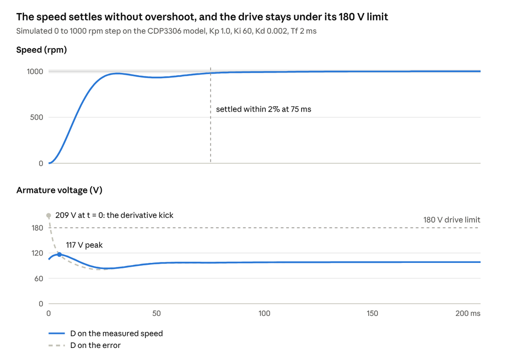

The speed rises in 19 ms, settles within 2% in 75 ms and never overshoots, so REQ-01, REQ-02 and REQ-03 pass. The voltage panel shows why the derivative sits on the speed. With the same gains applied to the error, the setpoint step asks for 209 V at t = 0, more than the drive can deliver. With D on the measured speed, the peak is 117 V and REQ-05 passes with margin.

Robustness and sample time

A good step response isn’t enough on its own, so check the loop’s margins too. The phase margin is 76° at a crossover of 89 rad/s, which passes REQ-04. The gain margin is infinite, because the phase never crosses −180°. Without the filtered D, the same PI gains give about 65°.

The controller will run on a microcontroller, so test it at the rate it will actually run. Discretize the controller with Tustin and the plant with a zero-order hold, which is how the processor sees it:

Ts = 0.001
motor_d = ct.c2d(motor_sys, Ts, 'zoh')     # plant as the MCU sees it
C_pi_d  = ct.c2d(C_pi, Ts, 'tustin')
H_d_d   = ct.c2d(H_d, Ts, 'tustin')
closed_d = ct.feedback(C_pi_d * ct.feedback(motor_d, H_d_d), 1)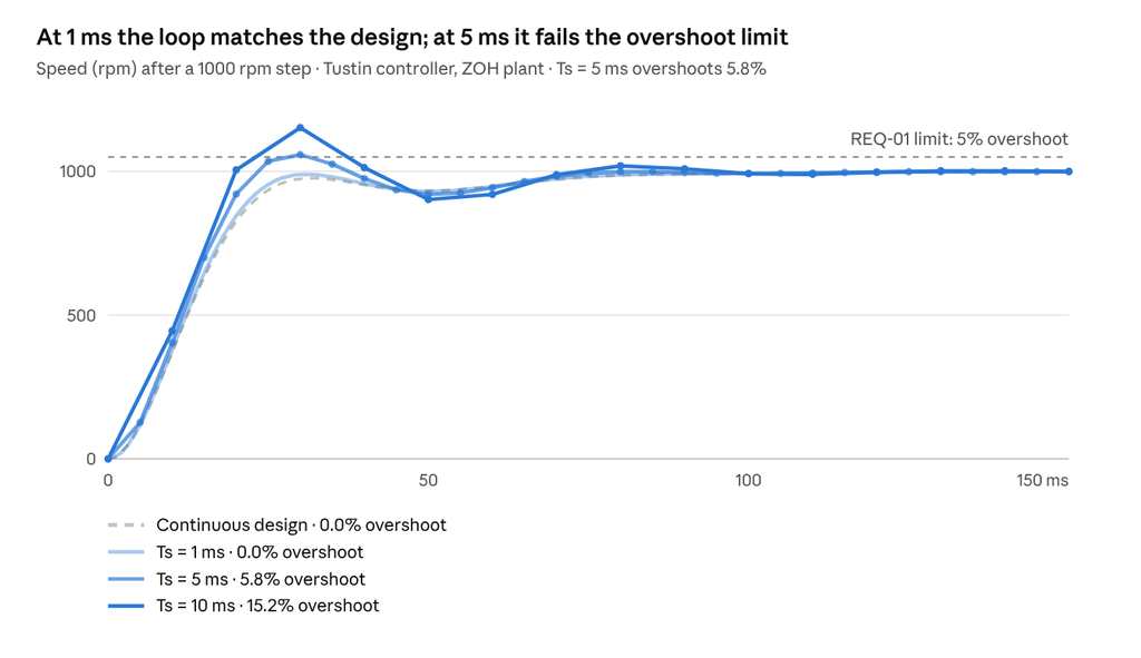

Sampling and the zero-order hold add roughly ωc·Ts/2 of phase lag. At 1 ms that is about 2.5° and the discrete loop matches the design. At 5 ms it is about 13°, enough to push overshoot past the 5% limit. The sample time is a design parameter, not an afterthought.

Requirements as tests

Each requirement becomes a pytest that imports the results from the script (saved as motor_pid.py):

# test_requirements.py
from motor_pid import info, pm, volts

def test_REQ_01_overshoot():
    assert info["Overshoot"] <= 5.0

def test_REQ_02_settling_time():
    assert info["SettlingTime"] <= 0.100

def test_REQ_03_steady_state_error():
    assert abs(info["SteadyStateValue"] - 1.0) < 1e-3

def test_REQ_04_phase_margin():
    assert pm >= 60.0

def test_REQ_05_voltage_limit():
    assert volts.max() <= 180.0

$ pytest -q
.....                                                    [100%]
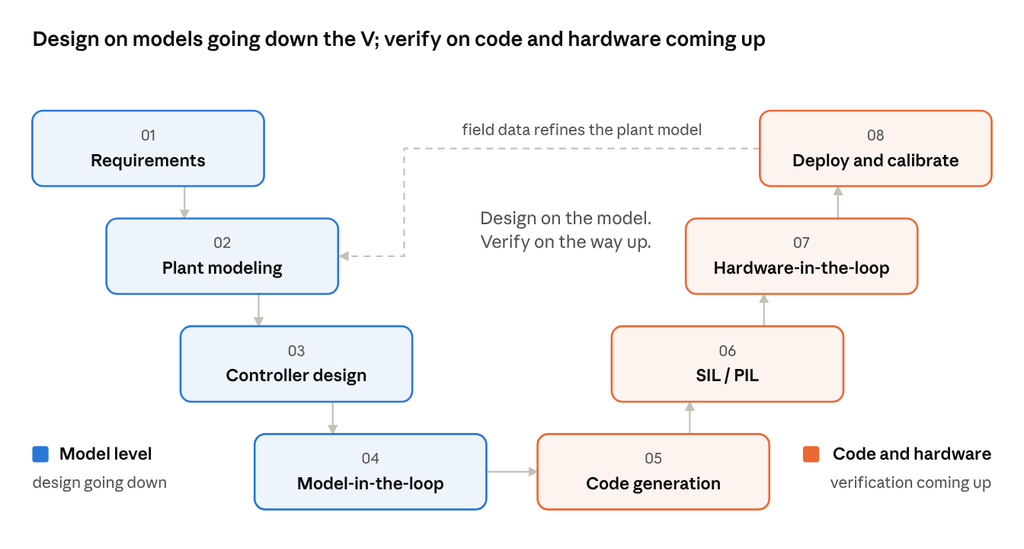
5 passed

Run this on every commit. If you change a gain or the sample time, the failing test tells you which requirement broke. That turns model-in-the-loop simulation into a regression suite for free.

Summary

Step	Result
Datasheet to model	K, R, L, J and b, each traced to a datasheet line
Model validation	1828 rpm predicted vs 1830 rpm measured
Controller	PI on the error (Kp 1.0, Ki 60), filtered D on the speed (Kd 0.002, Tf 2 ms)
Step response	0% overshoot, 75 ms settling, 19 ms rise
Robustness	76° phase margin, infinite gain margin
Actuator demand	117 V peak, under the 180 V limit
Sample time	1 ms, Tustin
Verification	5 requirement tests, all passing

These results use typical datasheet values. Next in the series, we read a Bode plot properly, then loop-shape this same motor. Later, we’ll identify the real motor from measured data and see how far the datasheet was off.

Have you ever caught a datasheet error that would have broken your design? Tell us in the comments, and follow Quadyne for the rest of the series.

A PID controller acts on three views of the same error: its size now (P), its history (I) and its rate of change (D). Getting the gains right is only half the job. Real hardware adds actuator limits, sensor noise and sampling, and each one breaks the textbook law in a predictable way.

This post covers what each term does, how to tune them, and the fixes that turn the textbook equation into firmware you can trust. It is the long-form companion to our Instagram carousel on the same topic.

The control law: three terms, one output

The controller acts on the error e = r − y, the gap between the reference r and the measured output y, and sums three contributions:

PID sums three views of the error into one actuator command

That is the parallel form. Many tools use the standard form instead, so check which one yours uses before copying gains:

The two are related by Ki = Kp / Ti and Kd = Kp · Td, so the same numbers give very different controllers in the two forms.

What each term does

P, the present. The output scales with the current error: a bigger error means a harder push. Higher Kp speeds up the response and shrinks the steady-state error, but on its own it never removes it on a plant without an integrator. Push Kp too far and the loop oscillates, then goes unstable.

I, the past. The integral accumulates error over time and keeps pushing until the error reaches zero. It eliminates steady-state error for constant setpoints and disturbances, but it adds phase lag. Too much Ki brings overshoot and slow oscillation, and with actuator limits, windup.

D, the future. The derivative reacts to how fast the error is changing, braking before the output overshoots. It adds phase lead and damping, so you can run higher gains with less overshoot. It also amplifies sensor noise, so always filter it, for example Kd·s / (1 + Tf·s) with Tf ≈ Td / N and N between 5 and 20.

In short, P sets the speed, I removes the offset at the cost of phase margin, and D buys damping.

What each gain changes

This table shows the classic trade-offs when you increase one gain and hold the others fixed.

Increase	Rise time	Overshoot	Settling time	Steady-state error
Kp	Faster	More	Small change	Less
Ki	Faster	More	Longer	Eliminated
Kd	Minor change	Less	Shorter	No effect

These are typical trends on well-behaved plants. Delays and nonlinearities change the picture, and the effects interact, so use the table to choose which knob to turn first and retune one gain at a time. One trade-off holds almost everywhere: anything that adds speed usually costs overshoot.

Four ways to tune

The methods range from quick tests on the plant to model-based design. Start from one, then finish by verifying the result.

Method	How it works	Trade-off
Ziegler–Nichols	Raise Kp until the loop oscillates steadily, giving the ultimate gain Ku and period Tu. Then Kp = 0.6 Ku, Ti = Tu/2, Td = Tu/8.	Fast, but aggressive: expect large overshoot and detune from there.
Lambda / IMC	Fit a first-order-plus-dead-time model K·e^(−θs)/(τs + 1). For PI: Kp = τ / (K(λ + θ)), Ti = τ.	One knob, λ, trades speed for robustness.
Relay autotuning	Relay feedback forces a small limit cycle, revealing Ku ≈ 4d/(πa) and Tu.	Finds Ku and Tu without driving the loop unstable.
Loop shaping	With a model, tune on the Bode plot for a target crossover frequency and phase margin.	Predictable robustness, but needs a model.

In the relay formula, d is the relay amplitude and a is the amplitude of the resulting oscillation. If you have a model, or can fit one, IMC and loop shaping give the most predictable robustness.

The pitfall: integral windup

When the actuator saturates, the integrator keeps charging on error the actuator can no longer act on. Once the output finally catches up, that stored integral has to unwind, which causes large overshoot and slow recovery.

There are three standard fixes:

• Conditional integration (clamping): stop integrating while the actuator is saturated.
• Back-calculation: feed the difference between the saturated and unsaturated output back into the integrator, with tracking time Tt.
• Limiting the integrator state directly.

Any PI or PID controller with actuator limits needs one of them.

From textbook to firmware

The textbook law has three terms; a practical discrete PID takes eight lines. This version runs once per sample time Ts:

e      = r - y
P      = Kp * (b*r - y)                          // setpoint weight b
I      = I + Ki*Ts*e
D      = a*D - Kd*(1-a)/Ts * (y - y_prev)        // filtered, on y
u_raw  = P + I + D
u      = clamp(u_raw, u_min, u_max)
I      = I + (Ts/Tt) * (u - u_raw)               // back-calculation
y_prev = y

Here a = Tf / (Tf + Ts), where Tf is the derivative filter time constant and Tt is the anti-windup tracking time.

• Derivative on measurement avoids a kick when the setpoint steps. The setpoint weight b softens overshoot without detuning disturbance rejection.
• Sample fast enough: roughly 4–10 samples per closed-loop rise time.
• Add bumpless transfer between manual and automatic modes.

Cheat sheet: which term fixes what?

Symptom	First thing to try
Response too slow	Increase Kp
Steady-state offset	Add or increase Ki
Overshoot or ringing	Add Kd, or reduce Kp
Slow oscillation	Reduce Ki
Noisy, chattering actuator	Filter the D term, reduce Kd
Big overshoot after saturation	Add anti-windup

What’s next

Next in the series, we build a PID in Python with open-source tools, on a real motor: the ABB Baldor-Reliance CDP3306.

What’s your go-to tuning method: Ziegler–Nichols, IMC, autotuning, or trial and error? Tell us in the comments, and follow Quadyne for the rest of the series.

Previous post:

Model-Based Controller Development: From Requirements to Real Hardware

Model-based development takes a controller from requirements to real hardware in eight stages, and it catches most problems before any hardware is at risk. You design against a model of the system, then verify the same design again at every step as it turns into code and runs on real electronics.

This post walks through those eight stages. It is written for practicing control engineers and graduate students, and it is the long-form companion to our Instagram carousel on the same topic.

The V-model at a glance

Design on models going down the V; verify on code and hardware coming up

The left side of the V designs on models; the right side turns the design into code and checks it on progressively more real hardware. Field data from deployment flows back into the plant model, so each project starts the next one with a better model.

Going down the V: design on the model

The first four stages happen entirely in software, on models. Mistakes here are cheap to fix.

1. Requirements

Turn system goals into measurable, testable control specs. Every requirement should link to a test case, because that link is what the right side of the V verifies against.

Category	What to specify
Time domain	Rise time, settling time, overshoot, steady-state error
Frequency domain	Bandwidth, gain margin (e.g. ≥ 6 dB), phase margin (e.g. ≥ 45°), noise and disturbance rejection
Constraints	Actuator limits, sample rate, CPU and memory budget, safety and fault behavior

Specify robustness, not just nominal performance: parameter variation, sensor noise and disturbances. Define the operating envelope and how the system must behave when things fail. The margin values above are common rules of thumb; use your domain’s targets.

Output: a requirements set, traceable to test cases.

2. Plant modeling

Model the physical system accurately enough for control design, and no more. There are three routes:

• White-box: physics, from conservation laws, Newton and Kirchhoff.
• Black-box: system identification from test data (step, chirp, PRBS).
• Grey-box: a physics structure with parameters fitted to data.

Validate the model against measured data you did not use for fitting. Include actuator and sensor dynamics, delays, saturation and quantization, since they often limit the bandwidth you can achieve. Linearize at operating points for design, but keep the nonlinear model for verification.

Output: a validated nonlinear model plus linearized design models.

3. Controller design

Choose a control law and tune it against the plant model. Common choices are PID with loop shaping, LQR/LQG, MPC, H∞ robust control and gain scheduling.

• Judge robustness, not just the step response: check margins and peak sensitivity Ms across model variations.
• Discretize for the target sample time (ZOH or Tustin) and account for the phase lag it adds.
• Design for reality: anti-windup, rate limits, saturation and bumpless mode transfer.

Output: a discrete-time controller model that meets the specs.

4. Model-in-the-loop (MIL)

Run the controller and plant models together in closed-loop simulation. This is the first verification gate, and no hardware is involved yet.

• Run the requirement-based test cases against the full nonlinear plant model.
• Sweep uncertainty with Monte Carlo runs, and stress edge cases such as saturation, sensor faults and large disturbances.
• Measure model coverage to find logic paths no test has exercised.

Output: a verified model, plus reference results for the back-to-back tests that follow.

Coming up the V: verify on code and hardware

The last four stages turn the model into code and move it onto real electronics. Each test layer makes one more part real, so a failure points to what just changed.

Test layer	Controller runs as	Plant is	What it catches
MIL	Model, on the desktop	Model	Design errors, requirement violations
SIL	Generated code, compiled on the host PC	Model	Code generation and data-type issues
PIL	Generated code, on the target processor	Model	Compiler, word-length and numerical issues; execution time and memory
HIL	Production code on the real controller, with real I/O	Real-time simulator	I/O, drivers, interrupts, timing, bus communication, fault handling
Deployment	Production code on the real controller	The real system	Anything left, under real operating conditions

5. Code generation

Generate embedded C/C++ automatically from the verified model, with no hand-coding: the model is the source. The generator needs a target configuration that sets data types, fixed-point scaling and task rates.

• Fix data types early. If the target has no FPU, use fixed-point scaling and check for overflow and precision loss.
• Apply a coding standard such as MISRA C, and run static analysis on the generated code.
• Keep bidirectional traceability: requirement ↔ model ↔ code.

Output: production code, plus traceability and analysis reports.

6. Software- and processor-in-the-loop (SIL & PIL)

Prove the generated code behaves exactly like the model. Run a back-to-back test: feed identical stimuli to the code and the model, and compare outputs against defined numerical tolerances.

• SIL compiles the code on the host PC and catches code-generation and data-type issues.
• PIL runs it on the target processor, adding the real compiler and CPU. It exposes word-length and numerical issues that the host PC hides.
• Profile execution time and stack and memory use on the target, against the real-time budget.

Output: model–code equivalence, plus a timing and memory profile.

7. Hardware-in-the-loop (HIL)

The real controller hardware drives a plant model running on a real-time simulator, connected through real I/O such as analog signals, PWM, encoders and CAN or EtherCAT.

• HIL exercises what simulation can’t: real I/O, drivers, interrupts, timing and bus communication.
• Inject faults safely: open circuits, stuck sensors, bus errors and extreme operating points.
• Automate regression suites so every software change is verified again.

Output: integrated controller software, verified before it touches the real plant.

8. Deployment and calibration

Close the loop on the real system and fine-tune in place.

• Commission in stages: start with conservative gains and safety limits, then widen the operating envelope.
• Tune parameters live through a calibration protocol such as XCP, without reflashing.
• Feed measured field data back into the plant model, so the next iteration starts closer to reality. This loop returns you to stage 2.

Output: a calibrated controller running on the real system.

Why go model-based?

Four things make the extra structure worth it:

• Catch errors early. Design flaws surface in simulation, long before they can damage hardware or reach the field.
• One source of truth. The same model drives design, code generation and test. Nothing is re-implemented by hand.
• Layered verification. MIL, SIL, PIL and HIL each re-check the previous stage on more realistic hardware.
• End-to-end traceability. Every requirement links to model elements, generated code and the tests that prove it.

What’s next

This post is the map for our series. Next, we break down PID control, then rebuild this whole workflow with open-source tools on a real motor, the ABB Baldor-Reliance CDP3306.

Which stage takes the most time in your workflow? Tell us in the comments, and follow Quadyne for the rest of the series.