Model-based development takes a controller from requirements to real hardware in eight stages, and it catches most problems before any hardware is at risk. You design against a model of the system, then verify the same design again at every step as it turns into code and runs on real electronics.
This post walks through those eight stages. It is written for practicing control engineers and graduate students, and it is the long-form companion to our Instagram carousel on the same topic.
The V-model at a glance
Design on models going down the V; verify on code and hardware coming up
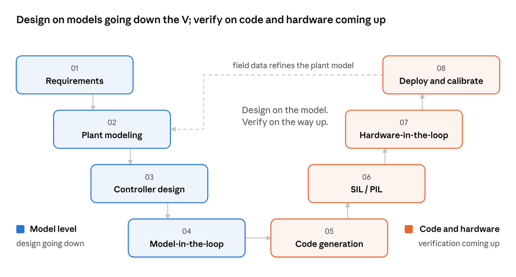
The left side of the V designs on models; the right side turns the design into code and checks it on progressively more real hardware. Field data from deployment flows back into the plant model, so each project starts the next one with a better model.
Going down the V: design on the model
The first four stages happen entirely in software, on models. Mistakes here are cheap to fix.
1. Requirements
Turn system goals into measurable, testable control specs. Every requirement should link to a test case, because that link is what the right side of the V verifies against.
| Category | What to specify |
|---|---|
| Time domain | Rise time, settling time, overshoot, steady-state error |
| Frequency domain | Bandwidth, gain margin (e.g. ≥ 6 dB), phase margin (e.g. ≥ 45°), noise and disturbance rejection |
| Constraints | Actuator limits, sample rate, CPU and memory budget, safety and fault behavior |
Specify robustness, not just nominal performance: parameter variation, sensor noise and disturbances. Define the operating envelope and how the system must behave when things fail. The margin values above are common rules of thumb; use your domain’s targets.
Output: a requirements set, traceable to test cases.
2. Plant modeling
Model the physical system accurately enough for control design, and no more. There are three routes:
- White-box: physics, from conservation laws, Newton and Kirchhoff.
- Black-box: system identification from test data (step, chirp, PRBS).
- Grey-box: a physics structure with parameters fitted to data.
Validate the model against measured data you did not use for fitting. Include actuator and sensor dynamics, delays, saturation and quantization, since they often limit the bandwidth you can achieve. Linearize at operating points for design, but keep the nonlinear model for verification.
Output: a validated nonlinear model plus linearized design models.
3. Controller design
Choose a control law and tune it against the plant model. Common choices are PID with loop shaping, LQR/LQG, MPC, H∞ robust control and gain scheduling.
- Judge robustness, not just the step response: check margins and peak sensitivity Ms across model variations.
- Discretize for the target sample time (ZOH or Tustin) and account for the phase lag it adds.
- Design for reality: anti-windup, rate limits, saturation and bumpless mode transfer.
Output: a discrete-time controller model that meets the specs.
4. Model-in-the-loop (MIL)
Run the controller and plant models together in closed-loop simulation. This is the first verification gate, and no hardware is involved yet.
- Run the requirement-based test cases against the full nonlinear plant model.
- Sweep uncertainty with Monte Carlo runs, and stress edge cases such as saturation, sensor faults and large disturbances.
- Measure model coverage to find logic paths no test has exercised.
Output: a verified model, plus reference results for the back-to-back tests that follow.
Coming up the V: verify on code and hardware
The last four stages turn the model into code and move it onto real electronics. Each test layer makes one more part real, so a failure points to what just changed.
| Test layer | Controller runs as | Plant is | What it catches |
|---|---|---|---|
| MIL | Model, on the desktop | Model | Design errors, requirement violations |
| SIL | Generated code, compiled on the host PC | Model | Code generation and data-type issues |
| PIL | Generated code, on the target processor | Model | Compiler, word-length and numerical issues; execution time and memory |
| HIL | Production code on the real controller, with real I/O | Real-time simulator | I/O, drivers, interrupts, timing, bus communication, fault handling |
| Deployment | Production code on the real controller | The real system | Anything left, under real operating conditions |
5. Code generation
Generate embedded C/C++ automatically from the verified model, with no hand-coding: the model is the source. The generator needs a target configuration that sets data types, fixed-point scaling and task rates.
- Fix data types early. If the target has no FPU, use fixed-point scaling and check for overflow and precision loss.
- Apply a coding standard such as MISRA C, and run static analysis on the generated code.
- Keep bidirectional traceability: requirement ↔ model ↔ code.
Output: production code, plus traceability and analysis reports.
6. Software- and processor-in-the-loop (SIL & PIL)
Prove the generated code behaves exactly like the model. Run a back-to-back test: feed identical stimuli to the code and the model, and compare outputs against defined numerical tolerances.
- SIL compiles the code on the host PC and catches code-generation and data-type issues.
- PIL runs it on the target processor, adding the real compiler and CPU. It exposes word-length and numerical issues that the host PC hides.
- Profile execution time and stack and memory use on the target, against the real-time budget.
Output: model–code equivalence, plus a timing and memory profile.
7. Hardware-in-the-loop (HIL)
The real controller hardware drives a plant model running on a real-time simulator, connected through real I/O such as analog signals, PWM, encoders and CAN or EtherCAT.
- HIL exercises what simulation can’t: real I/O, drivers, interrupts, timing and bus communication.
- Inject faults safely: open circuits, stuck sensors, bus errors and extreme operating points.
- Automate regression suites so every software change is verified again.
Output: integrated controller software, verified before it touches the real plant.
8. Deployment and calibration
Close the loop on the real system and fine-tune in place.
- Commission in stages: start with conservative gains and safety limits, then widen the operating envelope.
- Tune parameters live through a calibration protocol such as XCP, without reflashing.
- Feed measured field data back into the plant model, so the next iteration starts closer to reality. This loop returns you to stage 2.
Output: a calibrated controller running on the real system.
Why go model-based?
Four things make the extra structure worth it:
- Catch errors early. Design flaws surface in simulation, long before they can damage hardware or reach the field.
- One source of truth. The same model drives design, code generation and test. Nothing is re-implemented by hand.
- Layered verification. MIL, SIL, PIL and HIL each re-check the previous stage on more realistic hardware.
- End-to-end traceability. Every requirement links to model elements, generated code and the tests that prove it.
What’s next
This post is the map for our series. Next, we break down PID control, then rebuild this whole workflow with open-source tools on a real motor, the ABB Baldor-Reliance CDP3306.
Which stage takes the most time in your workflow? Tell us in the comments, and follow Quadyne for the rest of the series.