A PID controller acts on three views of the same error: its size now (P), its history (I) and its rate of change (D). Getting the gains right is only half the job. Real hardware adds actuator limits, sensor noise and sampling, and each one breaks the textbook law in a predictable way.
This post covers what each term does, how to tune them, and the fixes that turn the textbook equation into firmware you can trust. It is the long-form companion to our Instagram carousel on the same topic.
The control law: three terms, one output
The controller acts on the error e = r − y, the gap between the reference r and the measured output y, and sums three contributions:
PID sums three views of the error into one actuator command
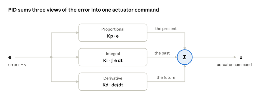
That is the parallel form. Many tools use the standard form instead, so check which one yours uses before copying gains:
The two are related by Ki = Kp / Ti and Kd = Kp · Td, so the same numbers give very different controllers in the two forms.
What each term does
P, the present. The output scales with the current error: a bigger error means a harder push. Higher Kp speeds up the response and shrinks the steady-state error, but on its own it never removes it on a plant without an integrator. Push Kp too far and the loop oscillates, then goes unstable.
I, the past. The integral accumulates error over time and keeps pushing until the error reaches zero. It eliminates steady-state error for constant setpoints and disturbances, but it adds phase lag. Too much Ki brings overshoot and slow oscillation, and with actuator limits, windup.
D, the future. The derivative reacts to how fast the error is changing, braking before the output overshoots. It adds phase lead and damping, so you can run higher gains with less overshoot. It also amplifies sensor noise, so always filter it, for example Kd·s / (1 + Tf·s) with Tf ≈ Td / N and N between 5 and 20.
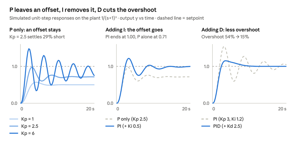
In short, P sets the speed, I removes the offset at the cost of phase margin, and D buys damping.
What each gain changes
This table shows the classic trade-offs when you increase one gain and hold the others fixed.
| Increase | Rise time | Overshoot | Settling time | Steady-state error |
|---|---|---|---|---|
| Kp | Faster | More | Small change | Less |
| Ki | Faster | More | Longer | Eliminated |
| Kd | Minor change | Less | Shorter | No effect |
These are typical trends on well-behaved plants. Delays and nonlinearities change the picture, and the effects interact, so use the table to choose which knob to turn first and retune one gain at a time. One trade-off holds almost everywhere: anything that adds speed usually costs overshoot.
Four ways to tune
The methods range from quick tests on the plant to model-based design. Start from one, then finish by verifying the result.
| Method | How it works | Trade-off |
|---|---|---|
| Ziegler–Nichols | Raise Kp until the loop oscillates steadily, giving the ultimate gain Ku and period Tu. Then Kp = 0.6 Ku, Ti = Tu/2, Td = Tu/8. | Fast, but aggressive: expect large overshoot and detune from there. |
| Lambda / IMC | Fit a first-order-plus-dead-time model K·e^(−θs)/(τs + 1). For PI: Kp = τ / (K(λ + θ)), Ti = τ. | One knob, λ, trades speed for robustness. |
| Relay autotuning | Relay feedback forces a small limit cycle, revealing Ku ≈ 4d/(πa) and Tu. | Finds Ku and Tu without driving the loop unstable. |
| Loop shaping | With a model, tune on the Bode plot for a target crossover frequency and phase margin. | Predictable robustness, but needs a model. |
In the relay formula, d is the relay amplitude and a is the amplitude of the resulting oscillation. If you have a model, or can fit one, IMC and loop shaping give the most predictable robustness.
The pitfall: integral windup
When the actuator saturates, the integrator keeps charging on error the actuator can no longer act on. Once the output finally catches up, that stored integral has to unwind, which causes large overshoot and slow recovery.
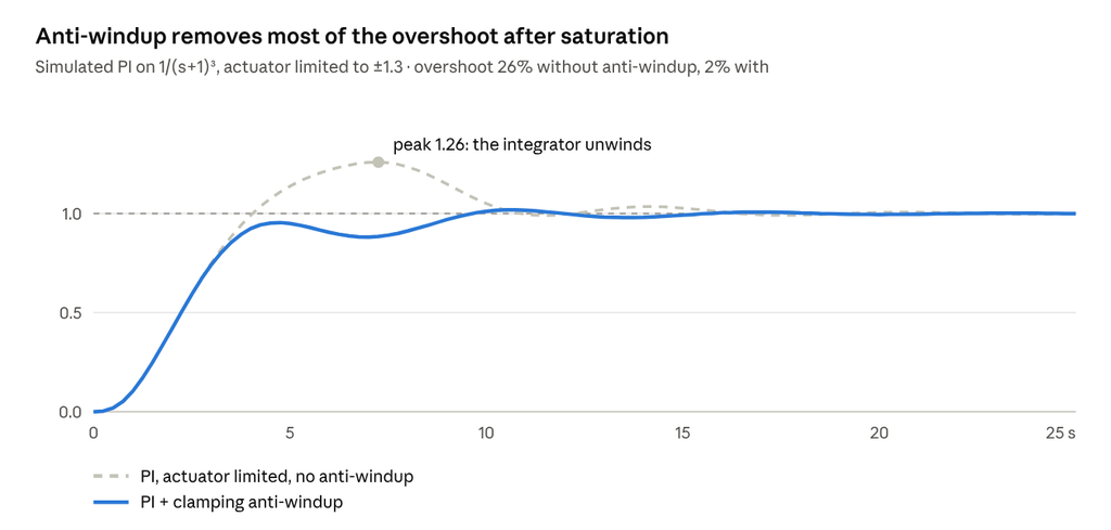
There are three standard fixes:
- Conditional integration (clamping): stop integrating while the actuator is saturated.
- Back-calculation: feed the difference between the saturated and unsaturated output back into the integrator, with tracking time Tt.
- Limiting the integrator state directly.
Any PI or PID controller with actuator limits needs one of them.
From textbook to firmware
The textbook law has three terms; a practical discrete PID takes eight lines. This version runs once per sample time Ts:
e      = r - y
P      = Kp * (b*r - y)                          // setpoint weight b
I      = I + Ki*Ts*e
D      = a*D - Kd*(1-a)/Ts * (y - y_prev)        // filtered, on y
u_raw  = P + I + D
u      = clamp(u_raw, u_min, u_max)
I      = I + (Ts/Tt) * (u - u_raw)               // back-calculation
y_prev = y
Here a = Tf / (Tf + Ts), where Tf is the derivative filter time constant and Tt is the anti-windup tracking time.
- Derivative on measurement avoids a kick when the setpoint steps. The setpoint weight b softens overshoot without detuning disturbance rejection.
- Sample fast enough: roughly 4–10 samples per closed-loop rise time.
- Add bumpless transfer between manual and automatic modes.
Cheat sheet: which term fixes what?
| Symptom | First thing to try |
|---|---|
| Response too slow | Increase Kp |
| Steady-state offset | Add or increase Ki |
| Overshoot or ringing | Add Kd, or reduce Kp |
| Slow oscillation | Reduce Ki |
| Noisy, chattering actuator | Filter the D term, reduce Kd |
| Big overshoot after saturation | Add anti-windup |
What’s next
Next in the series, we build a PID in Python with open-source tools, on a real motor: the ABB Baldor-Reliance CDP3306.
What’s your go-to tuning method: Ziegler–Nichols, IMC, autotuning, or trial and error? Tell us in the comments, and follow Quadyne for the rest of the series.
Previous post: